Oscilloscope Music
I recently came across an interesting art project called "Oscilloscope Music" by Jerobeam Fenderson:
Here's another excellent example by Chris Allen:
The video shown above is an XY trace taken on an oscilloscope which is being fed a carefully crafted audio file. The oscilloscope is drawing a single bright point of light, with the left audio channel controlling the X axis position of that point and the right audio channel controlling the Y axis position. Varying the amplitude of those two channels together allows that point of light to be used as a pen, drawing shapes on the 2D screen. You can find a much more detailed explanation of what's going on here from Smarter Every Day.
As soon as I saw this, I immediately wanted to see if I could recreate the same kind of visualization from that same audio. I do have an oscilloscope, but it's all the way in the other room, so I decided to see if I could recreate the result in code.
To do that, I started up Julia 1.4 and created the Jupyter notebook you see here.
Goals
My goal here is to take the audio track from a source like this video as input and recreate the video, showing the result you would see by playing that audio file into the X and Y channels of an oscilloscope.
Approach
To do this, I'm going to emulate the behavior of the oscilloscope trace. I'll start off with a black canvas. At each audio sample, I'll use the left and right channel amplitudes to pick an X and Y coordinate in that canvas, and I'll make that pixel white. This is basically what the oscilloscope does in XY mode: it is always drawing a bright dot, and the X and Y channels determine where that dot is.
You'll notice from all the oscilloscope music videos, however, that you can see more than just a single dot at a time. In fact, you can see smooth lines that don't seem to be made up of individual points. This happens because the oscilloscope display itself has some persistence. An electron beam is used to illuminate a single point on the screen, but when that beam moves elsewhere, it takes some time for the previous point to fade to black. Furthermore, if the beam is quickly moved across an area, the whole path of the beam will be illuminated and will only slowly fade back to black. We'll have to be careful to replicate that persistence when we digitally recreate the effect.
Code
To start off, we'll need to import a few Julia packages to handle our various inputs and outputs:
# WAV.jl lets us read .wav format audio files
using WAV: wavread

# Images and ImageMagick handle loading and working with images
using Images
using ImageMagick

# ProgressMeter lets us use `@showprogress` to turn a loop
# into a progress var
using ProgressMeter: @showprogress

# We'll use FFMPEG to strip the audio out of the Youtube video
using FFMPEG

# For...you know...plots
using Plots
Reading Audio Data
The source I'll be working with is "Blocks" by Jerobeam Fenderson. I've already downloaded the full video file using youtube-dl`:
video_file = "Jerobeam Fenderson - Blocks-0KDekS4YUy4.webm";
We only need the audio from that file, so I'll use FFMPEG to strip out the audio and save it as blocks.wav:
@ffmpeg_env run(
    `$(FFMPEG.ffmpeg) -i $video_file -vn -ab 128k -ar 44100 -y blocks_audio.wav`)
We can read the audio input with wavread, which returns a matrix of samples. Each column of samples is one left/right audio channel.
samples, sample_freq = wavread("blocks_audio.wav");
Let's plot the first 1s of audio, just to see what it looks like:
# Samples from 0.0 to 1.0 seconds
sample_range = round.(Int, 1 .+ (0 * sample_freq : 1 * sample_freq))

plt = plot(sample_range, samples[sample_range, 1],
    label="Channel 1 (X)",
    xlabel="Sample index",
    ylabel="Amplitude"
    )
plot!(plt, sample_range, samples[sample_range, 2],
    label="Channel 2 (Y)")
We can get an idea of what the oscilloscope screen would look like by treating the two audio channels as the x and y components of a parametric plot:
plot(samples[sample_range, 1], samples[sample_range, 2],
    legend=nothing)
This doesn't look anything like the original video, however, because it's missing the persistence effect I mentioned earlier. To look like an oscilloscope output, we need the result to slowly decay to black over time after the X and Y inputs change.
We'll handle that in the render function in the next section...
Rendering the Video
The add_sample! function mimics the behavior of the oscilloscope. It takes an image (a matrix of colors) called img, and channel values c1 and c2, both of which will be in the range [-1, 1]. It then finds the appropriate pixel in img, where c1=-1, c2=-1 would be the lower left corner and c1=1, c2=1 would be the upper right corner, and it sets that pixel to 1 (white).
This is essentially what the XY-input does in the oscilloscope: it causes the elctron beam to move to the given XY coordinates and illuminates that location on the screen.
function add_sample!(img::AbstractMatrix, c1::Number, c2::Number)
    img[round(Int, size(img, 1) / 2 - c2 * (size(img, 1) - 2) / 2),
        round(Int, size(img, 2) / 2 + c1 * (size(img, 2) - 2) / 2)] = 1
end
The render function puts it all together: Given a .wav audio file, it generates an animated GIF showing what the oscilloscope screen would look like:
function render(wav_file, output_file;
        decay_interval=64,
        start_time=0, end_time=10, framerate=30)

    samples, sample_freq = wavread(wav_file)

    # Create our canvas as a black 400x400 image
    img = zeros(Gray{Float32}, 400, 400)

    frames = [img]
    interval = round(Int, sample_freq / framerate)
    start_sample = max(1, round(Int, start_time * sample_freq))
    end_sample = min(size(samples, 1), round(Int, end_time * sample_freq))

    # We need to simulate the persistence of the oscilloscope
    # screen. We can do that by decaying each pixel's brightness
    # towards zero by a small amount. For better accuracy, we
    # should do this for every audio sample, but that means
    # updating every element in the image 44000 times per second.
    # That's going to be pretty slow. Instead, we can decay the
    # pixels a little bit more every `decay_interval` audio
    # samples. It's not quite as accurate, but it's much faster.
    decay_rate = 0.9995^decay_interval

    # Here is where we iterate over each audio sample
    # (within a given time range)
    @showprogress for i in start_sample:end_sample
        if i % decay_interval == 0
            img .*= decay_rate
        end

        # Given the current left and right audio signals, make the
        # correct pixel in the canvas white.
        add_sample!(img, samples[i, 1], samples[i, 2])

        # Once we've processed enough samples to make up a new video
        # frame, add it to our vector of frames.
        if i % interval == 0
            push!(frames, copy(img))
        end
    end

    # The ImageMagick.jl package can save a collection of frames
    # into an animated GIF. ImageMagick needs the frames to be
    # represented as a 3D matrix, but we currently have a vector
    # of matrices.
    #
    # The `reduce` and `reshape` commands let us transform that
    # vector of matrices into the right 3D shape for ImageMagick.
    concatenated_frames = reshape(reduce(hcat, frames),
            (size(img, 1), size(img, 2), :))

    save(output_file, concatenated_frames, fps=framerate)
end
To run the function we just wrote, we just need to give it the input and output filenames. In this case, I'm also telling it to start rendering at the 0 second mark and stop at the 100 second mark:
render("blocks.wav", "blocks_rendered.gif",
    start_time=0, end_time=100)
Results
Here's the simulated oscilloscope output:
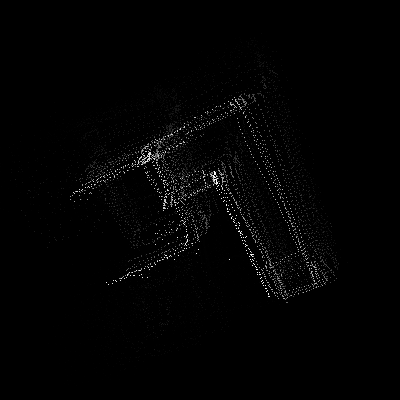
The result here isn't as crisp as you would see with a proper oscilloscope. I think the fuzziness is likely due to the audio compression of the source I started from (I don't have access to the uncompressed audio file, so I'm using the audio embedded in the original Youtube video).
Overall, though, I'm really happy with this result! It's a nice demonstration of moving back and forth between the audio and visual domains, and it proves that interesting data can hide anywhere.