Identifying Polygons with a Genetic Algorithm
Introduction
This post is about the process of creating a genetic algorithm-based system for identifying a polygon (determining its number of sides and their respective lengths) from a cloud of noisy data. This was nominally for a class I took, but mostly for my own enjoyment of the process of breaking down a really tricky problem into a bunch of solvable steps.
The Motivation
Last year, as part of a robotics class I was taking, my teammates and I were given a small robot equipped with a pair of touch sensors and sonar rangefinders (little devices that measure the distance to the nearest wall by recording the time it takes for a sonar pulse from the device to bounce back). Our job was to use the sonars to drive around an unknown obstacle and identify the number and length of each of the sides of that obstacle, in order to find out what shape it was. The algorithm that we were supposed to follow was, roughly, as follows:
- Drive at the obstacle until you crash
- When you hit the obstacle, use the touch sensors to line up the front of the robot to the side of the object
- Back up, turn 90 degrees.
- Using the sonars, scan backwards to the first corner of the obstacle you can find, then scan forward to the next corner.
- Follow the corner around until you crash into the obstacle again.
- Repeat until you’ve been all the way around the obstacle.
This seemed…inelegant for a number of reasons. First, the only method the robot had for determining its own position was odometry, that is, counting the number of turns of each of its wheels. Crashing into a wall tends to result in wheels slipping, which means that counting the number of wheel turns no longer tells you anything useful. Second, the whole crash-reverse-scan process was slow, and could take ten minutes or more for an obstacle only a few times the size of the robot. And finally, it just looked silly.
A Better Way
My teammates and I decided that we could do better. Instead of crashing into the obstacle over and over, we would just try to drive around the object, using the sonars to stay about a foot away at all times. Then, we could just use all the sonar data recorded by the robot to give us an idea of the shape and size of the obstacle. This broke the problem down into two sub-parts: wall-following and processing the sonar data.
Wall Following
Driving around the edge of the obstacle proved to be pretty straightforward. Our algorithm didn’t do much more than say “If you’re too close to the wall, turn away. If you’re too far away, turn to the wall.” By tuning the performance of that strategy, we were able to get the robot to drive around weirdly shaped objects like the one in this picture:
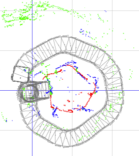
This is the image output by the simulator attached to our robot, which recorded data while the real robot was driving. The gray shapes are the robot’s estimated position at each time point (you can see where we bumped into the left side of the obstacle once). The red and blue dots represent individual sonar pings from our front and rear sonars, indicating an object of some kind at each dot. The green dots are sonar pings which reported an obstacle more than 1 meter away from the robot. We instructed the system to ignore those, since our sensors were nearly useless at that range.
What you see in the image is essentially a messy pentagon, composed of all the sonar data recorded by the robot. Once we had all that data, then, we needed to figure out what to do with it.
Identifying Polygons
Recording all of those sensor points was easy, but how to identify the shape and size of the real object those dots correspond to? This is, essentially, an example of “point cloud” analysis. We have a collection of dots which represent the outline of some shape, along with a lot of noise and error, and we need to extract the most likely shape from that cloud of points.
Now, extracting just a single line from a set of points is easy. We can just find the single line that minimizes the sum of the squared distance from each point to that line, using orthogonal regression, as shown in this image lovingly ripped off from Wikipedia:
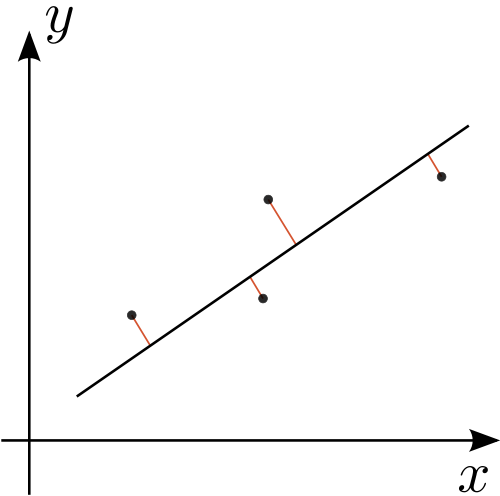
This is promising, but incomplete. Regression gives us a single line that fits our points, but it doesn’t work at all for shapes made up of multiple lines, and I’m not nearly enough of a mathematician to figure out how to extend the technique in that way.
What do we do?
Well, this idea of linear regression is still pretty appealing. In fact, if we could take all the points from the sonar data and figure out which ones corresponded to each edge of the obstacle, then we could just do regression on each set of points, which would give us the position of each of the edges. Then we can just find the intersection points of each of the edges to find the corners of the obstacle. Check it out:
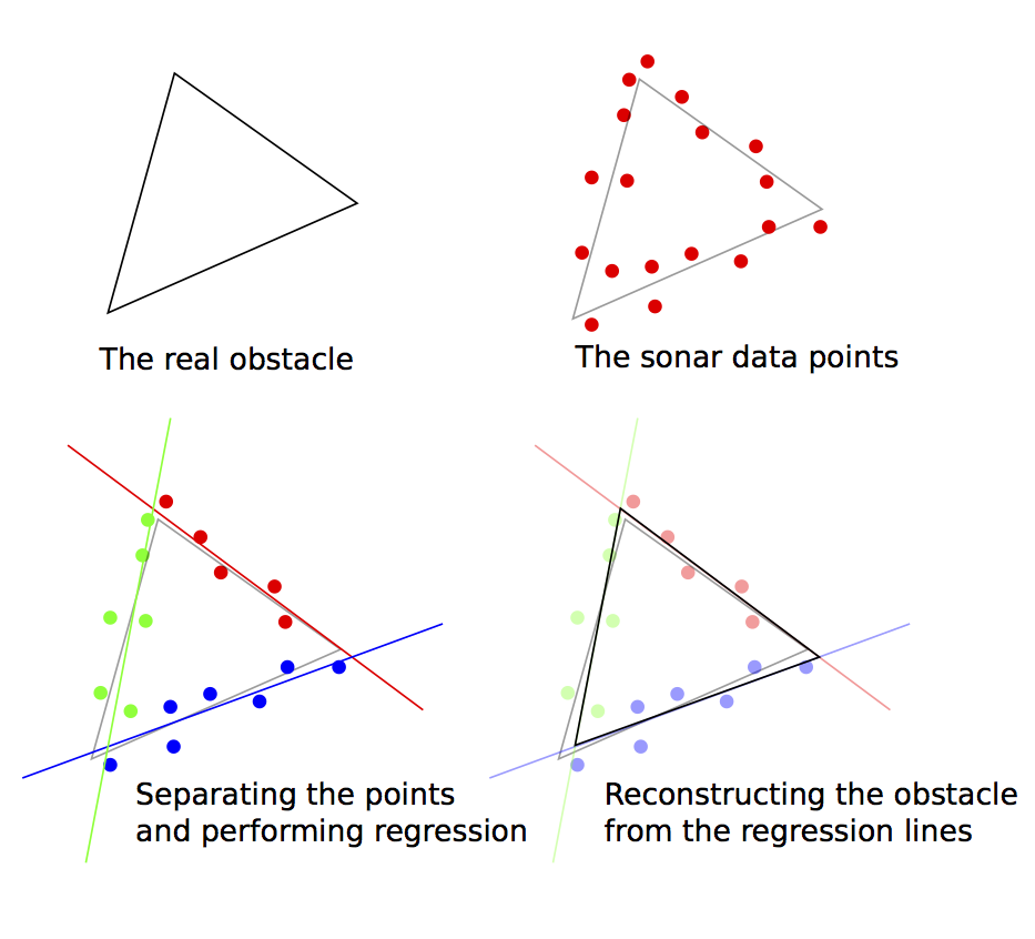
Cool. But this just creates another problem: How do we know how many edges there are, and which points correspond to which edge?
Segmenting the Point Cloud
Here’s where we are so far: We’ve started with a pretty complex problem of deriving the polygon that produced a particular point cloud of sonar data. By recognizing a parallel with a known, solved problem of regression, we’ve reduced it to a problem of dividing up our cloud into bins, each of which corresponds to a single edge of the polygon. Now we just have to figure out how to do that division cleverly.
The way I chose involves dividing the sonar points up by their angle relative to the centroid of the polygon. If the polygon were made of some flat material, then the centroid would be the point on which you could balance it perfectly. Of course, I don’t know what the real polygon is, just the sonar data, so I guesstimate that the centroid of the sonar data points (just the average of all their positions) is close enough.
For a three-sided shape I just choose three angles around the centroid, and use those angles to divide up the points. I can then do my orthogonal regression on the points in each section and re-derive the original shape. Of course, this relies on choosing the correct angles to divide up the shape. You can see two examples of choice of angles, one that divides the points up badly and gives us the wrong output shape, and one that divides them up well and gives us an excellent approximation of the original shape, here:
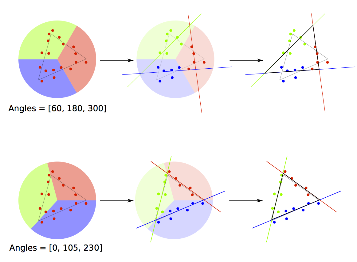
This hasn’t solved our polygon identification problem, but it’s further reduced it. Now we just need a way to choose three angles that give us the shape that best matches the sonar data.
Enter the GA
A genetic algorithm is an optimization technique which attempts to mimic the general process of evolution. “Optimization technique” just means that it’s a tool we can use to try to find the inputs to some mysterious function that produce the “best” output for a given problem. It’s “genetic” because it tries to find the best inputs to the function by simulating the life-and-death struggle of a “population” of inputs to our function, whose reproductive “fitness” is measured by how good the output they produce is.
The basic process is that we start out with a bunch of random inputs to try (maybe 10 or 20). We run the “fitness” function on all of those inputs, and we kill off, say, the half with the worst fitness values (side note: in optimization, we always talk about minimizing a function’s output by convention, so the best individuals are the ones with whom the fitness function produces the lowest output). We then take the remaining inputs, and perform reproduction and mutation on them. This just means that we take the “good” inputs and combine them with each other in some sensible way (perhaps just averaging two selected at random to produce a new input in between them), then we add some extra random change on top of that. This gives us a new crop of 10 or 20 individuals, so then we start over: killing the bad individuals, breeding the good ones, and so on.
I could pretend that I chose a GA for this problem because they’re particularly good at exploring really complicated fitness functions or because they have a lot of other cool engineering applications, but, to be honest, I just picked a GA here because I think they’re interesting and I wanted to try my hand at writing a nice implementation of one.
My GA Implementation
Each “individual” in our GA population is just a set of n angles, where n is the number of sides in our polygon. We measure the fitness of each individual by dividing up the sonar data according to those angles, performing regression on the points in each bin, and then summing the squared distance from each sonar point to the regression line it corresponds to. This means that if our regression lines fit all the sonar data very well, then we’ll get very low distances from all the sonar points, which gives us a very good fitness value.
We’ve now completely reduced this problem to a series of solvable steps: we use the GA to generate angles, we test them on our sonar data, and we eventually find the angles which give us the lowest total fitness value, and use those to generate the most likely polygon for our data.
Determining the Number of Sides
Actually, this was the easiest part of the entire problem. Given a set of points representing some unknown polygon, I just do the following:
Assume the shape has n sides (we start with n = 3) Run the GA with n angles, determine the total squared error of the best solution Now assume the shape has n+1 sides Run the GA again with n+1 angles, and determine the total squared error of the best solution If the total error has improved by 5% or more, then increment n and repeat the process. If the total error hasn’t improved by 5%, then the shape probably had n sides, so quit. This is based on a pretty simple observation, which is that 4 sides fit a rectangle much better than 3 sides do, but adding a 5th side won’t fit a square any better than 4 sides will. So we just add sides and keep trying until our performance stops improving. The magic 5% number was just chosen by trial-and-error.
Testing the GA
As it happened, we didn’t have time to do more than a couple of tests on the real robot. You can see two of them here:
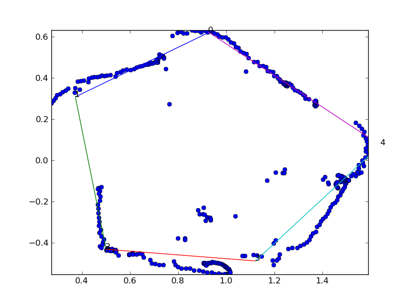
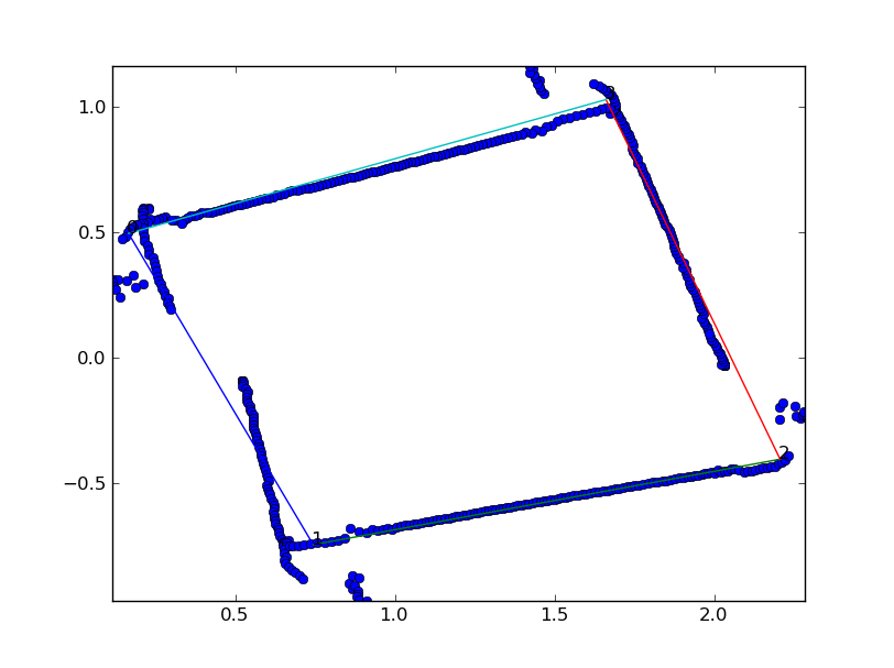
The blue points are all the sonar points (minus the ones the robot ignored, and the colored lines are the polygon sides that the GA determined. The gaps in the sonar data are the places where the robot crashed into the wall and had to re-align itself, and the sonar points don’t quite line up with each other due to error in the robot’s odometry data.
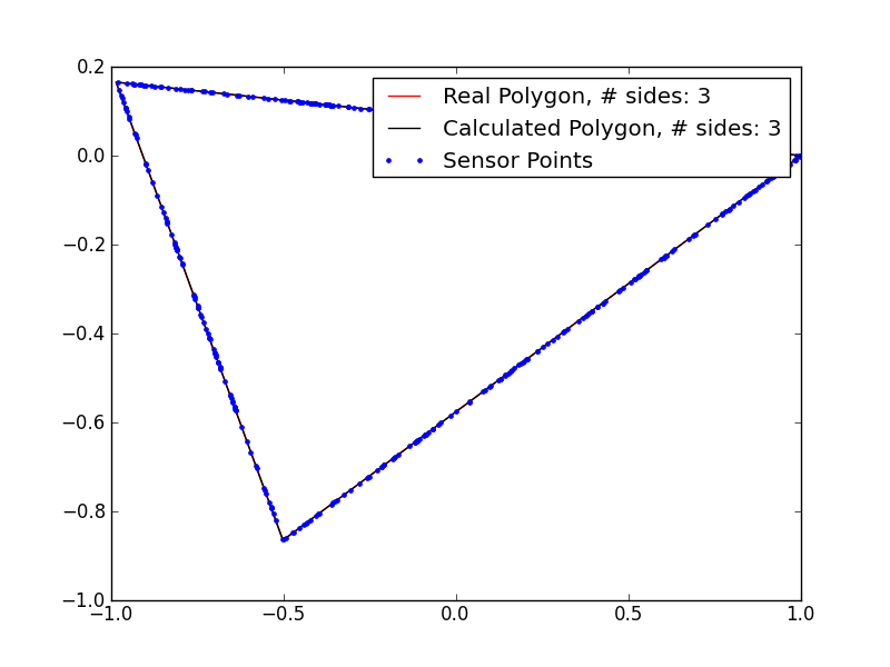
The rest of my testing was done on simulated data, since I no longer had access to the robot. To simulate data, I generated a random polygon with a random number of sides between 3 and 7, then generated 400 sonar points from that polygon, with a random, normally distributed, error added to each point. I could then run those points through my polygon identification GA and compare the real polygon to the one output by the GA. Here are a few examples:
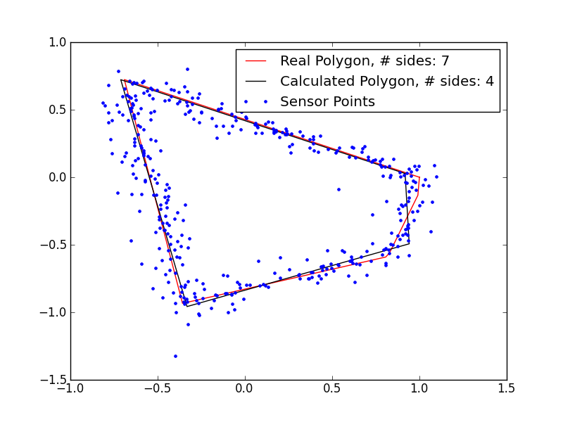
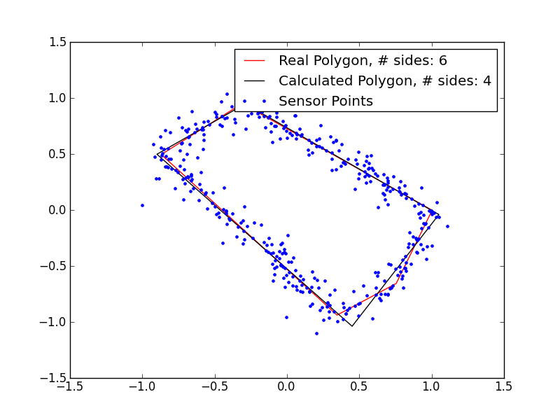
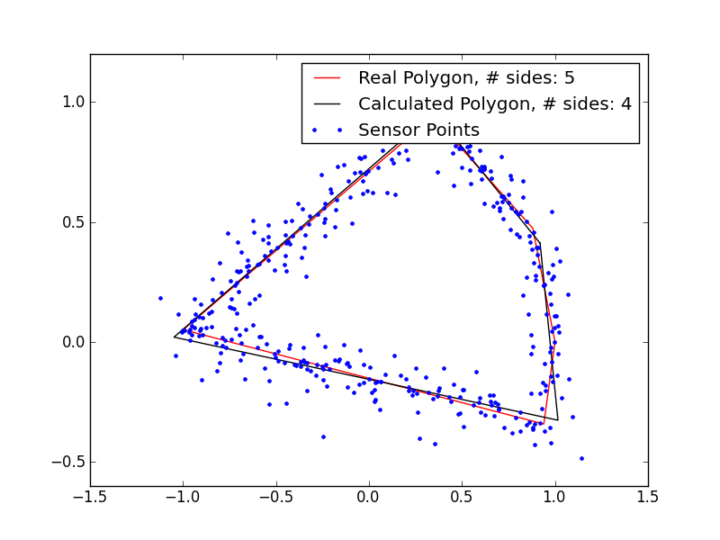
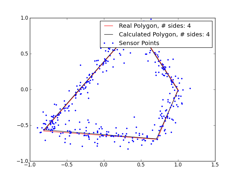
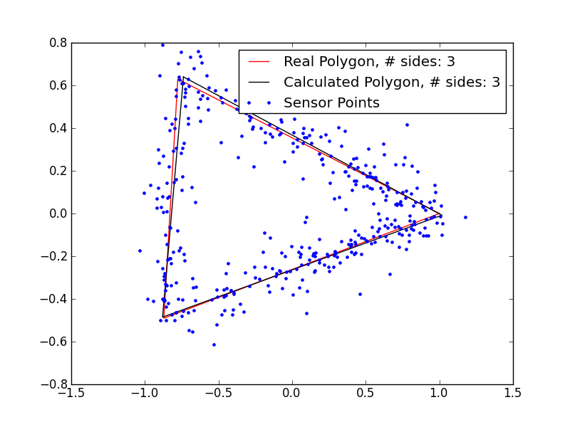
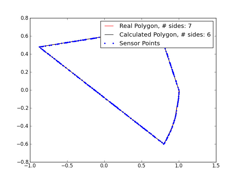
These results are pretty promising. I’m clearly underestimating the number of sides in the polygons with 5+ sides, so my magic number is probably not quite right, but even in those cases, I’m getting extremely close fits, despite the very noisy data. If I remove the noise, the fits are even better:
Of course, it wouldn’t be a genetic algorithm without occasionally producing a platypus or other crazy artifact of evolution:
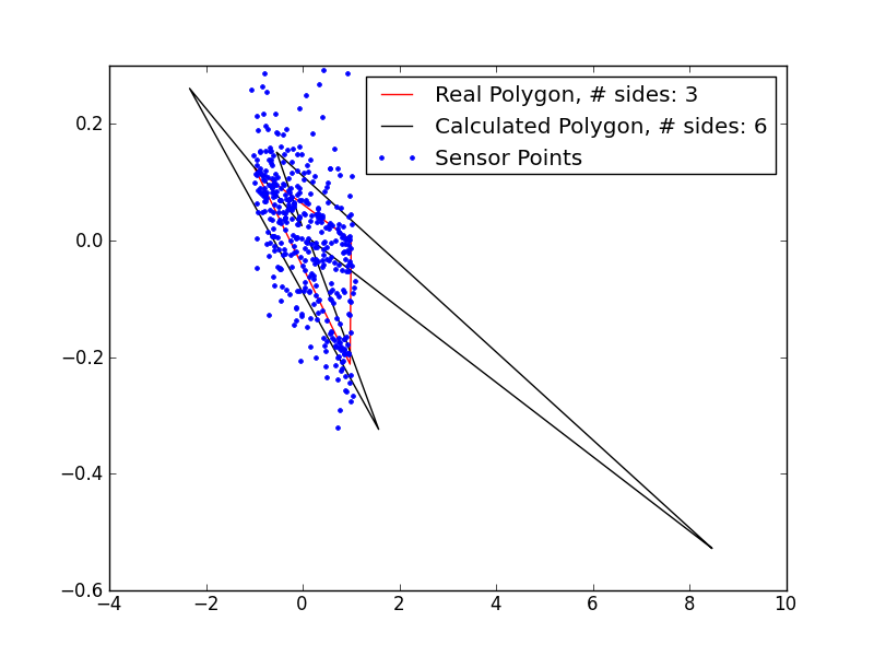
So, clearly there are some kinks to work out…
Try It Out
If you’d like to play with the software, it’s marginally useable and available on my github at rdeits/Identify-Polygons
Conclusions
I’m not rushing out to publish this as the latest advance in the field of computer modeling: it’s slow and somewhat unreliable and probably not the best solution for any particular problem. It was, however a lot of fun to do, and I hope it shows off just how cool optimization can be.
Robin Deits 20 February 2012